Unit II

Spatial Domain

Spatial domain processes involve direct pixel manipulation (point processing) of an image; it can be denoted by

$$g(x,y)=T[f(x,y)]$$

where $T$ is the spatial transform, $f$ is the input image, and $g$ is the output image.

Gary Level Transforms

In the following formulae

• $r⟶$ input pixel value
• $s⟶$ output pixel value
• $c⟶$ contrast
• ${\lambda }_{max}⟶$ maximum pixel value permissible by the image's datatype

Image Negative

Inverts the gray levels.

$s={\lambda }_{max}-r$

// For uint8 image
s = 255 - r

Log Transform

Spread/compresses the gray levels.

$s=c\cdot {\log }_{10}(1+r)$

s = c * Math.Log(1 + r);

Power Law Transform

Selectively increases/decreases the intensity of either dark/light pixels with minimum effect on the counterpart light/dark pixels.

$s=c\cdot r^{\gamma }$

s = c * Math.Pow(r, gamma);

• $\gamma >1⟶$ brightens image
• $\gamma =1⟶$ no change if $c=1$
• $\gamma <1⟶$ darkens image

Optimal Contrast

• The basic idea behind optimal contrast is to normalize the log and power law transforms to prevent overflow of values.
• This can be achieved by scaling up/down the entire image based on the fact that a ${\lambda }_{max}$ before transform should be same as ${\lambda }_{max}$ after the transform.
• Consider the following example

// Log transform
r = Math.Log(1 + 255);     // 2.408

// Power transform (low gamma, say 0.1)
r = Math.Pow(255, 0.1);    // 1.740

// Power transform (high gamma, say 2)
r = Math.Pow(255, 2.0));   // 65025

In all three cases, the output value becomes useless on the $[0,255]$ scale. To overcome this, we normalize the image.

// Log transform
c = 255 / Log(1 + 255);    // 105.886
s *= c;                    // 255 | Normalized

// Power transform (low gamma, say 0.1)
c = 255 / Pow(255, 0.1);   // 146.516
s *= c;                    // 255 | Normalized

// Power transform (high gamma, say 2)
c = 255 / Pow(255, 2.0);   // 0.00392
s *= c;                    // 255 | Normalized

Piecewise Transform

Contrast Stretching

This technique makes dark regions darker, and light regions lighter.

$r_1,r_2,s_1,s_2$ are selected as per preference. This results in three distinct regions where different transform slopes apply.

$$s=\{\begin{array}{ll}{m}_1\times r& r\le r_1\\ m_2\times (r-r_1)+s_1& r_1<r\le r_2\\ m_3\times (r-r_2)+s_2& r>r_2\end{array}$$

Solved Example Sample Problem

Thresholding

• In contrast stretching, if we make $r_1=r_2$, $s_1=0$, and $s_2={\lambda }_{max}$, we can create a threshold image based on the $\text{Threshold}=r_1=r_2$.

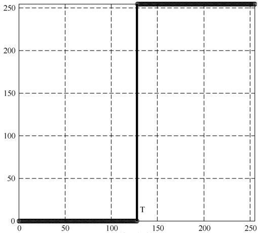
• Optimal threshold can be calculated by averaging the lightest and darkest pixel.

$\text{Threshold}=\frac{\text{Darkest Pixel + Lightest Pixel}}{2}$

• Furthermore, dividing the threshold image by ${\lambda }_{max}$ results in a binary/black-and-white image.

// Grayscale to logical conversion
image /= lambdaMax;

// For uint8 image
image /= 255;

Adaptive Thresholding

• Instead of globally applying the thresholding to the entire image at once, we can split the image into local sub-images/sub-matrices.
• Applying separate thresholding to separate regions will produce a better overall output in case of images with uneven illumination levels (one region is blown out, other is dim).

Gray Level Slicing

Highlight specific range $[A,B]$ of the graylevels.

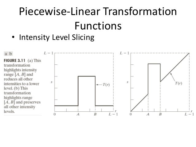
• It has two approaches
  1. Reduce graylevels outside of the range $[A,B]$.
  2. Preserve graylevels outside specified range $[A,B]$ i.e. do not change them.

Bit Plane Slicing

Highlight the contribution of specific or a range of bit planes.

• The most significant planes are the top 50% layers which contain visually significant data.
• It is useful in image compression (reducing number of gray levels) and filtering out most significant layers from an image.

• The number of bit planes depends on the bit-depth of the image.
• The leftmost bit is MSB, and therefore corresponds to the most significant plane.

Bit Plane Slicing CODE

image = Convert.ToDouble(uint3Image);

// Extract bits from image
layer1 = Floor(image / Pow(2, 0)) % 2; // least significant
layer1 = Floor(image / Pow(2, 1)) % 2;
layer1 = Floor(image / Pow(2, 2)) % 2; // most significant

// Recombine layers
recombinedImage = (2* (2 * (2 * layer3) + layer2) + layer1);

Histogram Sliding

Complete histogram is shifted right or left. This operation affects brightness.

// Right shift -> brighten image
image += shift

// Left shift -> darken image
image -= shift

NOTE

If the value of a pixel overflows or underflows after slide, it attains maximum or minimum value permissible in the datatype of image.

For example, in a uint8 image, data is bound by $[0,255]$

• $200+100=300$ $⟶$ overflow $⟶$ reset to ${\lambda }_{max}$
• $100-105=-5$ $⟶$ underflow $⟶$ reset to ${\lambda }_{min}$

Histogram Stretching

Stretch/compress the histogram to increase/decrease the contrast of the image.

• Map minimum value in histogram to ${\lambda }_{min}$
• Map maximum value in histogram to ${\lambda }_{max}$

$s=\frac{s_{max}-s_{min}}{r_{max}-r_{min}}\times (r-r_{min})+s_{min}$

// Stretch histogram in [10, 60] to occupy entire region [0, 255]
s = ((255 - 0) / (60 - 10)) * (r - 10) + 0

Solved Example Sample Problem

Histogram Equalization

• Although histogram stretching improves contrast, simply shuffling about the order of levels does not help much.
• To counter this, the histogram is then equalized/normalized/leveled using concept of cumulative sum.

Solved Example Sample Problem

Histogram Specification

• Although histogram equalization balances out the gray level, it has only one standardized out; no flexibility.
• Histogram specification adapts the balance one histogram based on an external histogram reference.

Solved Example Sample Problem

Mathematical Operations

Arithmetic Operations CODE

NOTE

Arithmetic operations can only be done on same size image/matrix.

% Crop image from top-left pixel
image = imresize(image, [100, 100]);

Arithmetic operations are simple element-to-element operation (hence same size matrices are required).

% Addition
result = imageA + imageB;

% Subtraction
result = imageA - imageB;

% Multiplication
result = immultiply(imageA, imageB);

% Division
result = imdivide(imageA, imageB);

% Invert
result = imcomplement(imageA);

Logical Operations CODE

NOTE

Logical operations can only be done on same size image/matrix.

Use the concept of optimal thresholding to convert an image from grayscale to binary.

% Crop image from top-left pixel
image = imresize(image, [100, 100]);

% Convert to logical image
optimalThreshold = (max(image) + min(image)) / 2
image = im2bw(image, optimalThreshold)

Logical operations are simple element-to-element operation (hence same size matrices are required).

% AND operation
result = imageA & imageB;

% OR operation
result = imageA | imageB;

% XOR operation
result = xor(imageA, imageB);

% NOT operation
result = ~image;                % !image in other languages
result = imcomplement(image);   % also works

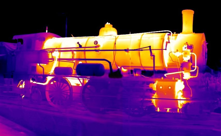
Pseudo Color

• Technique used to display images in color which were originally recorded in the visible or non-visible parts of the electromagnetic spectrum.
• Uses of pseudo color in visible spectrum
  • Change color temperature of an image
  • Map one spectrum of colors to another (eg: convert greens of an image to red)
  • Highlight key features of image

• Uses of pseudo color in non-visible spectrum
  • Map quantities such as radiation, heat, elevation, concentration (which don't have a color) to a spectrum in the visible region. This converts raw data to visual data which is easier to digest by humans.
  • Example: map the high infrared signals to red, and low infrared signals to blue. Image generated by such mapping will show hot areas in red, and cold areas in blue.

Color Image Enhancement CODE

RGB Colorspace

% Extract RGB components
rChannel = image(:, :, 1);  % red
gChannel = image(:, :, 2);  % green
bChannel = image(:, :, 3);  % blue

% Recombine
recombinedImage = cat(3, rChannel, gChannel, bChannel);

HSV Colorspace

% Convert to HSV colorspace
hsvImage = rgb2hsv(image);

% Extract HSV components
hChannel = hsvImage(:, :, 1);   % hue
sChannel = hsvImage(:, :, 2);   % saturation
vChannel = hsvImage(:, :, 3);   % vibrance

% Recombine
recombinedImage = cat(3, hChannel, sChannel, vChannel);

Using the same modification techniques used for grayscale, we can enhance the colored images by splitting them into different channels and applying enhancement techniques on them, and then recombining the channels.