Unit III

Spatial Filtering

• Image processing technique to reject certain frequency components.
• Involves usage of $n\times n$ filter mask which traverses through the image pixels.
• Advantage over frequency filters $⟶$ can also be used in non-linear domain.
• Types
  • Smoothening spatial filter
  • Sharpening spatial filter

Response of Linear Filter

$\text{Response}=\Sigma [w(i,j)\times f(x+i,y+j)]$

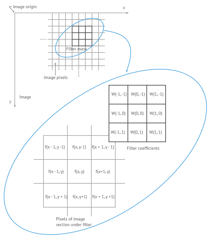
• $w(i,j)⟶$ weight of mask/filter
• $f(x+i,y+j)⟶$ corresponding image pixel
• After operation, $f(x,y)$ (center of mask) is replaced with with response.

NOTE

On the edges of an image, the row and/or column is mirrored appropriately to ensure proper filter operation. Defaulting it to 0 negatively affects the response on the edges.

Smoothening Spatial Filter

• Used in blurring and noise reduction. This process removes small, insignificant details from the image.

Average Filter

Takes the average of image matrix under the mask.

$$\frac{1}{9}\left[\begin{array}{ccc}1& 1& 1\\ 1& 1& 1\\ 1& 1& 1\end{array}\right]$$

Weighted Average Filter

Takes the weighted average of the image matrix under the mask. This gives us flexibility to give maximum weightage to the pixel being replaced i.e. center of the mask, and reduce weightage as we move away from the center.

Weighted average produces smoother output on detailed images with a lot of variation in vibrance region-to-region.

$$\frac{1}{16}\left[\begin{array}{ccc}1& 2& 1\\ 2& 4& 2\\ 1& 2& 1\end{array}\right]$$

Median Filter

Takes the median of values under the mask.

$\text{Response}=\text{Median}(f(x+i,y+j))$

Maximum Filter

Takes the maximum of values under the mask.

$\text{Response}=\text{Maximum}(f(x+i,y+j))$

Minimum Filter

Takes the minimum of values under the mask.

$\text{Response}=\text{Minimum}(f(x+i,y+j))$

Geometric Mean Filter

Takes the geometric mean of values under the mask.

$\text{Geometric Mean}=(x_1\times x_2\times \cdots \times x_n{)}^{\frac{1}{n}}$

$\text{Response}=\text{Geometric Mean}(f(x+i,y+j))$

Harmonic Mean Filter

Takes the harmonic mean of values under the mask.

$\text{Harmonic Mean}=\frac{n}{\frac{1}{x_1}+\frac{1}{x_2}+\cdots +\frac{1}{x_n}}$

$\text{Response}=\text{Harmonic Mean}(f(x+i,y+j))$

Sharpening Spatial Filter

• Used in sharpening, highlighting, and edge detection. This process highlights the sudden changes in H/S/V which usually happens at the edges of an object.
• Since we are dealing with sudden change in H/S/V, concept of derivative (rate of change) is very useful in sharpening filters.
• Since the values in an image are finite, the maximum change possible is ${\lambda }_{max}$ to ${\lambda }_{max}$ along adjacent pixels.
• In context of an image matrix
  • $f(x)⟶$ current pixel
  • $f(x+1)⟶$ next pixel
  • $f(x-1)⟶$ previous pixel

First Order Derivative Filter

Characteristics of first order derivatives

• Must be zero in flat segments
• Must be non-zero at onset of gray level ramp/change
• Must be non-zero along ramp

$\frac{df}{dx}=f(x+1)-f(x)$

Second Order Derivate Filter

Characteristics of second order derivatives

• Must be zero in flat area
• Must be non-zero at onset of gray level ramp/change
• Must be zero along ramp

$\frac{d^{2}f}{d{x}^2}=f(x+1)+f(x-1)-2f(x)$

Image Profile

• Edges are excluded because f′′ becomes undefined because there is no 'previous pixel'.
• The calculated derivatives follow the characteristics.

Conclusions from Image Profile

• $f\prime ⟶$ highlights thicker edges as it has non-zero response to ramps
• $f\prime \prime ⟶$ highlights finer details as it has strong response to isolated points

Laplacian Filter

• Works on principle of second order derivative filter.
• Since we'll use it on a mask, and not on a linear image profile, we have to modify the definition to include both $x-axis$ and $y-axis$.

$$\begin{gathered} f\prime \prime =\frac{{\partial }^{2}f}{\partial x^2}+\frac{{\partial }^{2}f}{\partial y^2} \\ \frac{{\partial }^{2}f}{\partial x^2}=f(x+1,y)+f(x-1,y)-2f(x,y) \\ \frac{{\partial }^{2}f}{\partial y^2}=f(x,y+1)+f(x,y-1)-2f(x,y) \\ f\prime \prime =f(x+1,y)+f(x-1,y)+f(x,y+1)+f(x,y-1)-4f(x,y) \end{gathered}$$

Mathematical Laplacian Mask

$$\left[\begin{array}{ccc}0& 1& 0\\ 1& -4& 1\\ 0& 1& 0\end{array}\right]$$

Modified Laplacian Mask

$$\left[\begin{array}{ccc}0& -1& 0\\ -1& 4& -1\\ 0& -1& 0\end{array}\right]$$

Continuous Laplacian Mask

$$\left[\begin{array}{ccc}-1& -1& -1\\ -1& 8& -1\\ -1& -1& -1\end{array}\right]$$

NOTE

In context of image processing, we want to give more weightage to the center pixel of the mask.

The mathematically derived Laplacian filter gives negative weightage to the center pixel, which is undesired. Therefore we multiply the mask by -1 to make it more suitable for digital image processing.

Highboost Filtering

• Sharpening by subtracting blurred image from original image.

// Highboost filter
sharpImage(x, y) = originalImage(x, y) - blurredImage(x, y)

Solved Example Sample Problem

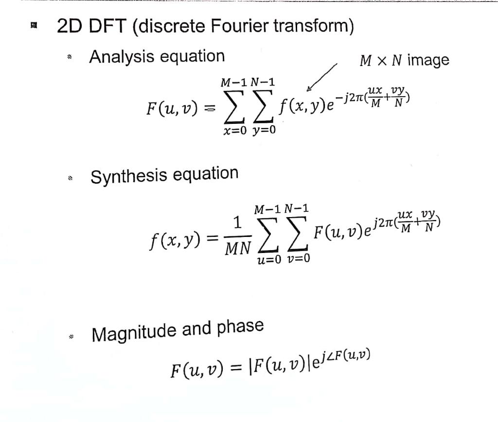
Image Enhancement in Frequency Domain

• Spatial domain (input) $⟶$ frequency domain (processing) $⟶$ spatial domain (output).
• Removes high or low frequencies.
• Change (function) is applied to entire image at once. There are no masks involved.

Fourier Transform

• Spatial domain $⟶$ frequency domain | DFT
• Frequency domain $⟶$ spatial domain | IDFT
• In context of DIP, we have to take two-dimensional Fourier transform

f(x, y)  ⇌  F(u, v)

Steps for Filtering in Frequency Domain

1. Preprocessing

// Input
f(x, y)

// Preprocessed input
f(x, y) * (-1)^(x + y)

2. Fourier transform

// Fourier transform using 2D DFT
F(u, v) = FourierTransform(f(x, y))

3. Filter in frequency domain

// Filter function
H(u, v)

// Apply filter function on image
G(u, v) = H(u, v) * F(u, v)

4. Inverse Fourier transform

// Inverse Fourier transform using 2D IDFT
g(x, y) = InverseFourierTransform(G(u, v))

5. Postprocessing

// Output
g(x, y)

// Postprocessed output
g(x, y) * (-1)^(x + y)

Filter Parameters

• D₀ $⟶$ non-negative constant to adjust the filter level
• D(u, v) $⟶$ distance from point (u, v)
• n is the sharpness of the filter. If n $\longrightarrow$ ∞, the filter becomes ideal.

// Distance function for an MxN image
D(u, v) = sqrt[ (u - M / 2)^2 + (v - N / 2)^2 ]

Notes on Usage of Frequency Filters

1. Ideal filters blur the edges of image.
2. Butterworth filters provide a smooth gradient at low sharpness n resulting in well defined edges.
3. Gaussian filters remove high/low frequency noise.

Smoothening Frequency Filter

• Utilizes lowpass filter to smoothen the image by removing the high frequency signals from the image.
• High frequency is basically noise and sudden changes in the image.

Ideal Lowpass Filter

// Filter function
H(u, v) = | 1   $\longrightarrow$   D(u, v) ≤ D₀
          | 0   $\longrightarrow$   D(u, v) > D₀

Butterworth Lowpass Filter

// Filter function
H(u, v) = { 1 + [D(u, v) / D₀]^2n }^(-1)

Gaussian Lowpass Filter

// Filter function
H(u, v) = e ^ { -D²(u, v) / (2 * D₀²) }

Summary

Sharpening Frequency Filter

• Utilizes highpass filter to sharpen the image by removing the low frequency signals from the image.
• Low frequency is basically continuity in the image. Continuity breaks at edges of an object.

Ideal Highpass Filter

// Filter function
H(u, v) = | 0   $\longrightarrow$   D(u, v) ≤ D₀
          | 1   $\longrightarrow$   D(u, v) > D₀

Butterworth Highpass Filter

// Filter function
H(u, v) = { 1 + [D₀ / D(u, v)]^2n }^(-1)

Gaussian Highpass Filter

// Filter function
H(u, v) = 1 - e ^ { -D²(u, v) / (2 * D₀²) }

Summary of Frequency Filters