Unit IV
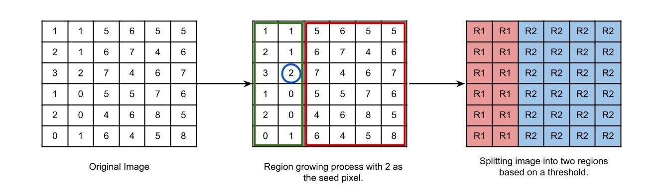
Image Segmentation
- Process of partitioning digital image into multiple region of interests (ROIs).
- Image segmentation approaches
- Similarity principle (region approach) group similar pixels to extract a coherent region
- Discontinuity principle (boundary approach) extract regions that differ in
H/S/V
Characteristics of Segmentation
- Similar pixels from an image region
Rare grouped into separate regions/subgroupsRᵢ
// Mathematical relation of ROIs
Σ Rᵢ = R
Rᵢmust be a connected region i.e.i = 1, 2, 3, ..., nRᵢs must be mutually exclusive region
// Mutually exclusive relation between Rᵢ and Rⱼ where i ≠ j
Rᵢ ∩ Rⱼ = ɸ
Predicate
P(Rᵢ)indicates some property over the regionRᵢ. Ideally, two different regions should have different predicates.Changing the tolerance of an ROI changes the shape of ROIs.
- Low tolerance will give accurate results, but may result in too many ROIs.
- High tolerance may give inaccurate results, but results in manageable number of ROIs.
Detection of Discontinuities
- Types of gray level discontinuities
- Point isolated point
- Line straight line
- Edge irregular outline of an object
Point Detection
- Isolated point whose gray level is significantly different from its background.
- If the response of a region is greater than or equal to the threshold, we can say an isolated point exists.
- This threshold is subjective non-negative integer, and its value depends on the application.
// Point detection mask
Mask = | -1  -1  -1  |
       | -1   8  -1  |
       | -1  -1  -1  |

// Isolated point condition
| R | ≥ T
Line of Detection
- There are four types of lines: horizontal, vertical, +45° diagonal, -45° diagonal.
- This means four types of masks are used for line detection.
// Horizontal line mask
Mask = | -1  -1  -1  |
       |  2   2   2  |
       | -1  -1  -1  |

// Vertical line mask
Mask = | -1   2  -1  |
       | -1   2  -1  |
       | -1   2  -1  |

// +45° Diagonal line mask
Mask = | -1  -1   2  |
       | -1   2  -1  |
       |  2  -1  -1  |

// -45° Diagonal line mask
Mask = |  2  -1  -1  |
       | -1   2  -1  |
       | -1  -1   2  |
- Response from all four line masks is calculated.
- The mask giving the highest response is associated with corresponding line.
Edge Detection
- An edge is a set of connected pixels which lie on the boundary of an object (boundary of two different).
- Edge corresponds to the sharp discontinuities/change in
H/S/Vand therefore can be used in segmentation. - Edge can extracted by computing the derivative of an image
- Magnitude of derivative contrast of edge
- Direction of derivative edge orientation (angle)
Types of Edges
- Step edge abrupt change in
H/S/V - Ramp edge gradual change in
H/S/V - Spike edge abrupt change in
H/S/Vand then back to originalH/S/V - Roof edge gradual change in
H/S/Vand then gradually back to originalH/S/V
Stages in Edge Detection
- Start
- Input image
- Filtering some preprocessing to aid in edge detection (smoothening, reduce noise)
- Differentiation first or second order derivative and direction if
atan(y / x) - Localization identify the edge location. Also involves edge thinning and edge linking.
- Display
- End
Edge Detection Approaches
- Derivative spatial filters
- Template matching matches region which resemble template
- Gaussian derivatives best for real time processing
- Pattern fit topographical surface generation
Edge Detection Techniques
First Order Edge Detection
// Edge magnitude
M = | Gx | + | Gy |

// Edge gradient (angle)
ϕ = tan⁻(Gy / Gx)

// Edge localization
| 1   $\longrightarrow$   M ≥ Threshold
| 0   $\longrightarrow$   M < Threshold
Robert Operator
- Mask is the derivative w.r.t. diagonal elements.
- Also known as cross diagonal difference.
// Robert Masks
GxMask = |  1   0 |
         |  0  -1 |

GyMask = |  0   1 |
         | -1   0 |
Prewitt Operator
- Central difference of neighboring pixels.
// Prewitt Masks
GxMask = | -1  -1  -1 |
         |  0   0   0 |
         |  1   1   1 |

GyMask = | -1   0   1 |
         | -1   0   1 |
         | -1   0   1 |

// Diagonal Prewitt Masks
GxMask = |  0   1   1 |
         | -1   0   1 |
         | -1  -1   0 |

GyMask = | -1  -1   0 |
         | -1   0   1 |
         |  0   1   1 |
NOTE
Which row/col is -ve doesn't really matter. What matters is row/col should have opposite signs to get the difference of neighboring pixels.
Conventionally, left/top side is taken as -ve and right/bottom side is taken as +ve.
For diagonal masks Gx is -45° and Gy is +45°.
Sobel Operator
- Central difference of neighboring pixels
- Also provides a smoothening effect
- First approximation of first Gaussian derivative
// Sobel Masks
GxMask = | -1  -2  -1 |
         |  0   0   0 |
         |  1   2   1 |

GyMask = | -1   0   1 |
         | -2   0   2 |
         | -1   0   1 |

// Diagonal Sobel Masks
GxMask = |  0   1   2 |
         | -1   0   1 |
         | -2  -1   0 |

GyMask = | -2  -1   0 |
         | -1   0   1 |
         |  0   1   2 |
Template Matching
- Direction sensitive filter.
- The masks can be obtained by rotating the matrix clockwise for a clockwise change in orientation.
- Also known as compass masks.
- The highest response corresponds to the direction of edge.
- Say,
M7 (South East ↙)gives highest response, then edge has a South East ↙ orientation.
Kirsch Mask
// M0 (East ←)
M0 = | -3  -3   5 |
     | -3   0   5 |
     | -3  -3   5 |

// M1 (North East ↖)
M1 = | -3  -3  -3 |
     | -3   0   5 |
     | -3   5   5 |

// ... ↑ ↗ → ↘ ↓

// M7 (South East ↙)
M7 = | -3   5   5 |
     | -3   0   5 |
     | -3  -3  -3 |
Robinson Mask
// M0 (East ←)
M0 = | -1   0   1 |
     | -2   0   2 |
     | -1   0   1 |

// M1 (North East ↖)
M1 = | -2  -1   0 |
     | -1   0   1 |
     |  0   1   2 |

// ... ↑ ↗ → ↘ ↓

// M7 (South East ↙)
M7 = |  0   1   2 |
     | -1   0   1 |
     | -2  -1   0 |
Second Order Edge Detection
- Zero crossing (crossing of second derivate from
+veto-veor vice versa) corresponds to edge. - So, if the response of filter changes sign, we can conclude an edge is present in the image.
- Unlike first order edge detection, second order is rotationally invariant.
Simple Laplacian Mask
// Laplacian filter
Mask = |  0  -1   0  |
       | -1   4  -1  |
       |  0  -1   0  |

// Continuous Laplacian filter
Mask = | -1  -1  -1  |
       | -1   8  -1  |
       | -1  -1  -1  |
Laplacian of Gaussian (LoG) Filter
- Also known as Marr-Hildrith filter.
- This filter accounts for variation in scale of image, and is capable of calculating both first and second order derivatives.
- Gaussian function reduces noise.
- To minimize noise susceptibility, LoG is preferred over simple Laplacian.

σdecides the size of the convolution mask generated.- Higher
σcorresponds to higher ordern x nfilter mask. - Higher
σgives better performance of the edge operator at cost of processing.
Difference of Gaussian (DoG) Filter
- Difference between two Gaussian filters with
σ₁andσ₂ - Ratio of
σ₁andσ₂between 1 and 2 is optimal.
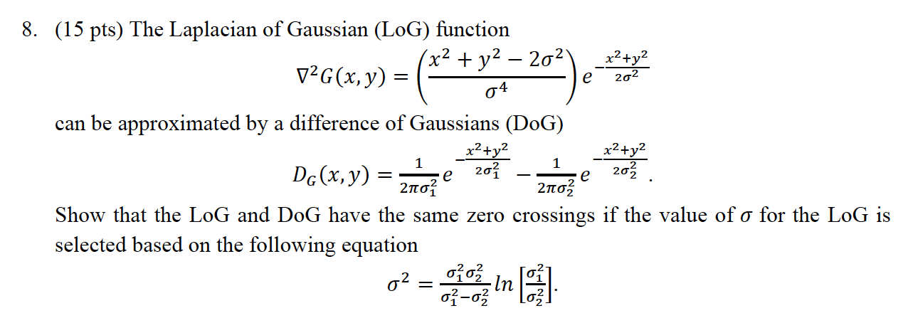
- Since DoG is an approximation of LoG and does not require Laplace transform, DoG is less resource intensive alternative to LoG.

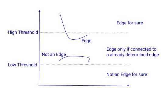
Canny Edge Detection
- Multistage algorithm to detect wide range of edges in an image.
- Multistage approach provides the benefit of
- Good edge detection with few false edges
- Good edge localization.
Canny Edge Algorithm
Preprocess smoothening
- Convolve image with Gaussian filter to produce a smooth image
- Compute gradient of result and store both magnitude and store
Mϕin separate arrays (see first order edge detection for more info).
Reduce the number of edges using non-maxima suppression
- Utilizes the concept of 'confidence' from fuzzy logic to eliminate regions with low confidence.
- This confidence threshold is a subjective choice.
Apply hysteresis thresholding
Segmentation using Watershed Segmentation
- Grayscale level of an image can be mapped as topology elevation.
- Raining on this topology forms water catchment basins.
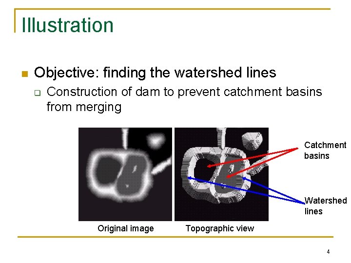
- Catchment basin (lake) collection of points where water will certainly fall to a unique regional minima.
- Watershed lines (boundary of lake) collection of points where water is equally likely to fall to more than one regional minima.
- If we can find the watershed lines, we can determine the edges. Here's a slice from the 3D plane we generated.

Basic Morphological Algorithms
Boundary Extraction
// Boundary by eroding the topology
B(A) = A - (A ⊖ B)
Solved Example Sample Problem
Region Filling
// Fill region by dilation the topology
Xₖ = (Xₖ₋₁ ⊕ B) ∩ Aʹ

// Structuring element B (constant)
B = | 0  1  0 |
    | 1  1  1 |
    | 0  1  0 |
- This process is repeated until
Xₖ == Xₖ₋₁
Solved Example Sample Problem
Extraction of Connected Component
// Fill region by dilation the topology
Xₖ = (Xₖ₋₁ ⊕ B) ∩ A

// Structuring element B (constant)
B = | 1  1  1 |
    | 1  1  1 |
    | 1  1  1 |
- This process is repeated until
Xₖ == Xₖ₋₁
Solved Example Sample Problem
Convex Hull
- Smallest possible polygonal hull (shape) to encapsulate the object.
// Convex hull formation by hit-or-miss of the topology
Xₖⁱ = (Xₖ₋₁ ⊗ Bᵢ) ∪ A

// Structuring element B (constant)
B1 = | 1  x  x |
     | 1  0  x |
     | 1  x  x |

// Rotate B1 clockwise **twice** to get B2, B3, and B4
- This process is repeated until
Xₖ == Xₖ₋₁
Solved Example Sample Problem
Thinning and Thickening
// Thinning
Thin(A, B) = A - (A ⊗ B)

// Thickening
Thick(A, B) = A ∪ (A ⊗ B)

// Structuring element B (constant)
B1 = | 1  x  0 |
     | 1  1  0 |
     | 1  x  0 |

// Rotate B1 clockwise **once** to get B2, B3, B4, B5, B6, B7, and B8
- If B mask matches the image
- If thinning, replace center by
0 - If thickening, replace center by
1
- If thinning, replace center by
- This process is exhaustive. Only one iteration is performed.
Solved Example Sample Problem
Homomorphic Filtering
- Homomorphic filtering simultaneously normalizes the brightness and increases the contrast.
Uses
- Correcting non-uniform illumination
- Removing multiplicative noise
- Appearance of grayscale image
Process
// Split image into illumination and reflectance
f(x, y) = i(x, y) x r(x, y)

// However, product of Fourier transform is not separable
F[f(x, y)] ≠ F[i(x, y)] x F[r(x, y)]

// To overcome, this problem, we preprocess the signal by taking its log
ln[f(x, y)] = ln[i(x, y)] + ln[r(x, y)]

// Fourier transform
F[ln[f(x, y)]] = F[ln[i(x, y)]] + F[ln[r(x, y)]]
- Illumination is the primary factor which provides image its dynamic range and it varies slowly.
- Reflectance is the detail of object edges and varies rapidly.
- These characteristics led to association of
F[f(x, y)]'s- Low frequencies with
F[i(x, y)] - High frequencies with
F[r(x, y)]
- Low frequencies with
- By applying separate filtering functions
HiandHrtoF[ln[i(x, y)]]andF[ln[r(x, y)]], we can achieve the primary function of homomorphic fiter.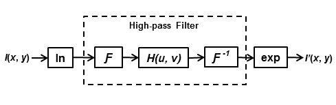
Image Restoration
- Process of removal of degradation in an image.
- Degradation is incurred during acquisition, transmission, or storage.
- Restoration is an objective process based on concrete, non-subjective mathematical models.
- Uses prior knowledge to achieve this.
- Causes
- Out of focus lens
- Atmospheric turbulence, mirage
- Improper ISO
Degradation Model

Original Image Degrade Function Degraded Image Add Noise Degrade Function Original Image Estimate
Restoration Techniques
- Inverse filtering
- Minimum mean squares filtering
- Constrained mean square filtering
- Non-linear filtering
Areas of Restoration
- Quantum limiting imaging in x-ray
- CT (computed tomography) scan in healthcare
- Image postprocessing in phone camera